TG A Changing Cosmos
{ All GSS Books }
~{}~
Objectives [] Assessment
Guides for each Chapter: 1 – 2 – 3 – 4 – 5 – 6 – 7 – 8 – 9
Goal 1: Students acquire beginning skills using HOU Image Processing software so they can start doing astronomy investigations.
- Objective 1A: Students can interpret graphs and alternate data representations, from pixels on an image to plotted data.
- Objective 1B: Students can measure sizes using Image Processing software toolsand compare sizes using ratios.
- Objective 1C: Students make systematic use of technology to enhance image features for classification purposes.
Goal 2: Students gain familiarity with celestial objects and comprehend the signficance of those objects in terms of layout of the Universe and our place in the Universe.
- Objective 2A: Students classify objects and identify trends and patterns within a data set.
- Objective 2B: Students can describe lunar surface features, galaxy types, and a range of objects in the universe.
- Objective 2C: Students can describe the phenomenon of supernovae.
- Objective 2D: Students compare sizes of features ranging from lunar craters to the diameter of galaxies.
Goal 3: Students use mathematics to solve practical problems in astronomical settings.
- Objective 3A: Derivation and application of functions and ratios within the context of a scientific technique.
- Objective 3B: Students can analyze complex systems involving multiple factors.
- Objective 3C: Students are familiar with the number scale and scientific notation, and use of appropriate units of measurement.
- Objective 3D: Interpretation and transformations among various data representations beginning with pixels on an image, leading to angular size and then to linear size.
- Objective 3E: Students use of ratios to convert from one type of measurement to another.
- Objective 3F: Students use geometry to derive, validate and apply the Small Angle Approximation.
~{}~
Objectives [] Assessment
Guides for each Chapter: 1 – 2 – 3 – 4 – 5 – 6 – 7 – 8 – 9
Assessment Tasks
General ideas for assessing student progress towards the goals and objectives of the GSS course are suggested in Part 6 of Basic GSS Overview.
Portfolios
We especially encourage the use of portfolios as a means of providing feedback to students and to demonstrate evidence of student progress to parents. Portfolios for A Changing Cosmos might include answers to the numbered questions posed in each chapter as well as written work done for each of the Investigations:
- Using Star Maps (chapter 2)
- CCD Camera Egg Carton Model (chapter 2)
- Browsing the Universe (chapter 2)
- Size and Scale of the Sun (chapter 3)
- Parallax (chapter 4)
- Inverse Square Law of Brightness (chapter 4)
- Star Magnitudes (chapter 4) Cepheids (chapter 4)
- Observing Color and Temperature (chapter 5)
- Measuring the Color of Stars (chapter 5)
- How Filters Work (chapter 5)
- HR Diagram of 47 Tucanae (chapter 5)
- Finding Supernovae (chapter 6)
- Eclipsing Binary Data Mining (chapter 6)
- Tracking Jupiter’s Moons (chapter 7)
- Finding Exoplanets (chapter 7)
In addition to portfolios, we suggest that you use assessment tasks both before and after presenting the unit. The papers that students’ complete before beginning the unit will help you diagnose their needs and adjust your plans accordingly. Comparing these papers to the students’ responses on the same tasks after completing the unit will allow you to determine how your students’ understanding and attitudes have changed as a result of instruction. Three tasks which we suggest be used for pre- and post- assessment are as follows:
- Questionnaire These questions are designed to determine how students’ knowledge of key concepts have changed during the unit, and whether or not they have changed their opinions concerning personal actions and environmental issues.
- Concept Map Asking students to create a concept map before and after the unit is one way to determine which concepts they have learned and their understanding of the connections among these concepts. If students have not had experience in concept mapping, you might want to start them out with a hand-out showing an example (master on p. 8), a general idea of what they are to map, and starting word(s) to help get them started. Once they have had experience with concept maps, they can create them on blank sheets of paper (no photocopying required). Alternatively, they can use concept mapping software such as
- Inspiration (http://www.inspiration.com)
- CMap (http://cmap.ihmc.us/conceptmap.html – free for noncommercial use).
- Omnigraffle (http://www.omnigroup.com/applications/omnigraffle Mac OSX)
- Freemind (http://freemind.sourceforge.net/wiki/index.php/
- Main_Page – open source software for mind-mapping.)
- Microsoft Draw (comes with Microsoft Office)
These two tasks fall along a spectrum from traditional to nontraditional ways of assessing student progress. The Questionnaire is a traditional way to elicit student understanding. It assesses students’ abilities to express themselves as well as insights that they gained from the unit. The Concept Map is nonlinear. Students do not need to think in terms of sentences and paragraphs, and their ideas can flow more freely. Students who are more visual might be better able to show what they know on this task than on the Questionnaire.
Interpreting Student Responses
The tasks should be interpreted in terms of the objectives listed in the Goals and Objectives state above. The Concept Map and Drawing Interpretation tasks are more loosely related to specific objectives. Comparing students’ papers before and after instruction may show that they have learned more about some objectives than others, or that certain misconceptions persist while others have been corrected. Eventually, we hope to be able to provide sets of instructions (called “rubrics”) to score student papers with respect to course objectives; but we do not yet have enough student data to do this.
In the meantime, we suggest that you pair students’ pre- and post-assessment papers and compare them.
With the list of objectives in mind, look for changes in the students’ attitudes and understanding. As you look through your students’ papers, you’ll be able to jot comments for individual students concerning main points they may have missed, or praising them for their insights and ideas. After looking over all of the papers you will be able to write down some generalizations about what the class as a whole learned or did not learn during the course. The three tasks are presented on the following pages. You may want to make two class sets of each of the tasks, using one color of paper for the pre-assessment measures and a different color of paper for the post-assessment measures.
Changing Cosmos—Concept Map
A concept map is a way of displaying your knowledge about a certain subject area. It consists of a set of words in boxes representing the most important ideas. The boxes are connected by lines and words showing how the ideas in the boxes are related. For example, at right is a concept map about the United States.
Your task is to create a concept map about the Universe. Your concept map should show ways of thinking about the Universe as a system. Start with the word “Universe” at the top. (If you’d like more space, you can draw your concept map on the back, or on another sheet of paper.)

Universe
Cosmic Change—Questionnaires
These .doc files contain questions that were developed by Kate Meredith, with substantive input from HOU staff and teachers, as well as input at annual HOU conferences. They are in four groups corresponding to key National Standards for Astronomy content in high school.
~{}~
Objectives [] Assessment
Guides for each Chapter: 1 – 2 – 3 – 4 – 5 – 6 – 7 – 8 – 9
Chapter-By-Chapter Suggestions
Before you start
At least a day or two before you begin A Changing Cosmos, distribute copies of the assessment tasks (see Assessment Tasks section) and ask your students to answer the questions. Explain that they will not be graded on these. The purpose is for them to show you what they already know so that you can plan the course accordingly.
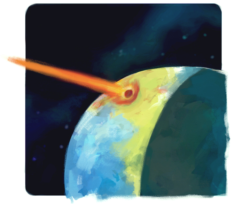
Chapter 1. Cosmic Cataclysms
This first chapter is mostly to just get students thinking about the cosmos in terms of events that could have real effects on their lives. You may choose to have a class discussion about students’ feelings about these sobering possibilities of disaster from cosmic origins.
Invite students to contribute their own knowledge and perspectives. Some might have read science fiction stories or seen movies that deal with some of these scenarios. Some may have read newspaper or magazine articles.
Have students to a web search for “SpaceGuard” to find out more about current searches for near-Earth asteroids.
There may be current Hands-On Universe high school student research in this field. See the HOU web site for latest info: http://handsonuniverse.org/usa/
Search for supernovae has also been an area of active HOU research by high school student teams. The HOU website will ahve news about any latest efforts in that area.
Construct a time line
It is always useful when dealing with geological ages to have a time line that will give the proper perspective of both human existence and the ages of the past. Have the student construct a time line on the chalkboard or a long sheet of butcher paper or masking tape placed on the wall. If the entire period of modern Homo Sapiens existed about 50 thousand years, and that is represented by 1 cm, then how far back on the time line did the dinosaurs become extinct? (65 million years ago, or 13 meters on the time line.) How long were the dinosaurs the dominant life form on the Earth? (For more than 150 million years, or 30 meters on the time line.)
The students can experiment to simulate crater production. Wet clay or plaster of Paris of the proper consistency can model the Earth’s surface. A large asteroid usually vaporizes after it strikes the surface. The students can experiment with drops of water, pebbles, balls of clay or pieces of plaster of Paris as simulations of an asteroid. Other possibilities include: splash water with hand; splash cornstarch mixture with hand. When a successful simulation is constructed, ask the students to vary the impact speed and examine the differences in the craters produced. Is there a relationship between the speed of their model asteroids and the size or shape of the craters?
Class Debate: Divide the class into two groups: the Volcano Theory supporters vs. the Meteor Impact Theory supporters. Each group must provide evidence in support of assigned theory. Have the two groups read this chapter, jotting down arguments for their theory and against the alternative theory. Provide time for them to collect further evidence on the debate at a library. Finally, allow for a timed debate between the two groups.
What is kinetic energy?
A briefing for advanced students
Derivation of the Equation for Kinetic Energy
Understanding the general idea of kinetic energy does not require any specialized knowledge; but understanding where the equation comes from involves some definitions.
Definition of average velocity (Vave ):
Vave = d/t
Velocity has the same definition as speed, but with the addition of direction. For a car moving at an average speed of 60 miles per hour, the above equation says that it would go a distance (d) of 60 miles in a time (t) of one hour.
When a large asteroid strikes the Earth, it is traveling at a very high initial velocity (VI). When it strikes the Earth, it slows down and comes to a stop. So, it’s final velocity (VF) equals zero. This is an important period of time, because it is while the asteroid is slowing down and coming to a stop that it transfers all of its kinetic energy to the Earth!
In order to estimate the kinetic energy of the asteroid we’ll assume that its average velocity— while the asteroid was ploughing into the crust and slowing down to a stop—was about one half of its initial velocity.
Vave= ½ (VI )
From these equations, we can find the distance that the asteroid travels into the crust:
d = ½(VI) t
Definition of acceleration (a)
a = (VF -VI ) / t
Acceleration means a change in speed. The most common example is a car, which might accelerate to 60 miles per hour in ten seconds. Its acceleration would be 6 miles per hour per second. The asteroid’s acceleration is negative instead of positive, since it is slowing down. And, its final velocity (VF) equals zero:
a = -VI / t
Definition of force (F) F = m a
Force (F) is a push or a pull, and it can be measured by a spring scale. Here on the Earth, if we do not exert a continuous force, objects slow down and stop. That’s because of friction. If we could eliminate friction completely, any force would make an object go faster and faster, as it is applied continuously. In space, for example, where there is no friction, if your rocket engines fire continuously, you will go faster and faster and faster. The above equation, known as Newton’s Second Law, says that a given force (F) applied to a given mass (m) will accelerate it at the rate (a). In a sense, this important equation defines what we mean by force.
Definition of work (W)
W = F d
It’s difficult to believe, but in physics, doing math problems is not considered real work, but playing basketball is! That’s because “work” has the special meaning of “force times distance.” When you are sitting at a table you are not going anywhere, so d = 0. But when you are playing basketball, you are exerting a force on an object (the ball, and yourself) that moves a measurable distance.
Definition of kinetic energy (E)
E = W
Energy of motion, or kinetic energy, is defined by the amount of work that an object can do on its surroundings. The asteroid is exerting a tremendous force when it collides with the Earth, and it continues to exert that force as long as it continues to plow through the crust. With the help of algebra that relates the above equations, we can find an equation that lets us estimate the energy by knowing the mass of the object and its velocity.
Start with: E = W = F d
Recall that:
1) F= ma
2) d = ½VI/t
3) a = VI/t
Substitute: E = F d = (ma) (½VI/t)
E = m (VI/t) (½VI/t) = ½mVI2
So, kinetic energy E = ½mVI2
where VI is the initial velocity of the asteroid before it begins to slow down, and m is its mass.
You may reinforce how the kinetic energy equation is used by having students do some problems that require its use.
~{}~
Objectives [] Assessment
Guides for each Chapter: 1 – 2 – 3 – 4 – 5 – 6 – 7 – 8 – 9
Chapter 2. Astronomers’ Tools
Investigation 2-1: Reading Star Maps
Uncle Al’s starwheels are practical tools for students to be able to find objects in the night sky. They also very useful for determing what objects are visible at a given time of year for students involved in research projects requiring requests for new images from HOU telescopes.
Answers to questions…
2.1 What Right Ascension line now points to the “S” in Southern Horizon? [correct answer 16]
2.2 What constellation just rose, almost due east? [Aquila or Capricorn]
2.3 What constellation is setting in the northwest? [Cancer and Gemini]
2.4 What constellation is closest to the zenith (highest place in the sky; center of the map)? [Draco, Bootes, or Hercules]
Rotate the Star Wheel FORWARD by another 2 hours.
2.5 What Right Ascension line now points to the “S” in Southern Horizon? [correct answer 18]
2.6 What constellation is closest to the zenith? [Draco, Lyra, or Hercules]
2.7 What constellation is rising, almost due east? [Aquarius]
2.8 What constellation is setting in the west? [Virgo or Corvus]
Rotate the Star Wheel FORWARD one last time by another 2 hours (30°).
2.9 What Right Ascension line now points to the “S” in Southern Horizon?
[correct answer 20]
2.10 What constellation is closest to the zenith? [Cygnus or Lyra]
2.11 What constellation is rising in the northeast? [Pisces or Cetus]
2.12 What constellation is setting in the northwest? [Virgo or Libra]
2.13 What constellation is near the zenith on New Year’s Eve at 11 pm? [Auriga]
2.14 In what month is the Big Dipper (Ursa Major) highest in the sky at midnight? [answer: March-April]
2.15 About what time is Leo setting (in the northwest) on the summer solstice (about June 21)? [between 11 pm and midnight]
2.16 How many degrees does the sky shift in one month? [30°]
You can opt to have students work in groups or pairs to make up more questions to challenge their partners to answer.
2.17 In which constellation is the Owl Nebula? [Ursa Major]
The HOU Messier Object Excel spreadsheets are kept at the Star Wheels page. You might choose to mark the BRIGHTEST Messier objects on your Coordinate Star Wheel, or perhaps the CLOSEST Messier objects.
In the “Moving Planets” section, you may want to point out that exceptions to the general west-to-east drift of the solar system objects (planets and asteroids) in their orbits occur when the Earth in its own orbit is “overtaking” an object, at which time the planet seems to move in the opposite direction (east to west). This reverse movement is called retrograde motion.
If you have your students use the JPL ephemeris generator, mentioned at the end of the investigation, any “Table Settings” are possible, but for your first ephemeris, keep it simple—check only #2 Apparent RA&DEC and possibly # 29 Constellation ID.
Investigation 2-2: CCD Image Color Coding
Tim Spuck, a TRA and high school teacher in Oil City Pennsylvania wrote this activity. The impact comes when students decide on their own Keys for coloring the grid and then all the sheets are displayed. Some color codes will bring out the detail of the spiral galaxy better than others will, and discussion about this can help in understanding what is happening when students use different lookup tables for color and different brightness/contrast Min/Max ranges.
Some teachers have suggested giving some of the students only 3 colors instead of 4.
The faint object at the top middle of the grid requires some sort of “log” scaling to bring out its detail.
Investigation 2-3: Browsing the Universe
• The Browsing the Universe investigation introduces various types of objects in the sky and encourages students to “play” with the software to create an image that is pleasing to them. It is particularly exciting, if a printer is available, for students to take home a copy of their work.
• The intent of this investigation is to have students discover the variety of different objects in the universe and explore questions about what they are and why they appear the way they do. Curiosity and hypotheses should be encouraged, and the inhibitions that are associated with “right” or “wrong” answers should be avoided. You can point out that no one is sure about the nature of astronomical objects, and even professional astronomers must start by “guessing” what they could be.
• In part I (Browsing), be sure that students understand that they should make a hypothesis about what type each object might be and why it looks the way it does, without doing any special research about the objects. One goal is for each student to ask “What is that object or feature ?” and choose to explore more about it.
• In part II (Galaxy Features), students need to do image processing to answer scientific questions about galaxy classification.
Galaxy types (common answers):
galaxy1 spiral
galaxy2 irregular or peculiar, possibly edge-on spiral
galaxy3 lower galaxy spiral, upper one debatable
galaxy4 elliptical
galaxy5 barred spiral
galaxy6 irregular or peculiar, possibly edge-on spiral
galaxy7 spiral
galaxy8 elliptical
• This is the first investigation using the Image Processing (IP) software (SalsaJ), so be sure to have computers available and allow adequate time for students to familiarize themselves with the software tools. SalsaJ is free software, downloadable from https://globalhandsonuniverse.org/software/
There is a manual there as well.
Tips about the IP software tools…
Image > Adjust Brightness/Contrast. Since the shades/colors are divided evenly over the range between Min and Max, narrowing the range brings out more detail within that brightness range, but loses all detail outside the range. Strategies for adjusting Min/Max to bring out detail usually start as trial and error. Often this is frustrating and provides the motivation for finding another way. Using cursor readings is another way. Sampling the brightness of background pixels is a way to determine a new Min above the brightness of background. To find a new value for Max, sample the brightness of bright object pixels. This will distribute all the colors or shades of grey over the range of interest
Zoom increases the size of each pixel, and at Zoom 4 or 5 the whole image does not fit on the screen, fewer pixels fit on the screen, and this means the dimensions of the screen in pixels is less. The dimensions of the image, however, remain the same, as can be seen by scrolling. A higher zoom does not change the overall size of the image in pixels; it just doesn’t all fit on the screen at the same time. Scrolling allows you to bring in the image, part by part, to check the pixel dimensions of the image.
Lookup Tables for Color. This question is included to provide an understanding of what the different colors or shades mean and how resolution depends upon the Min/Max range.
Plot Profile. The different high points in a Plot Profile graph mean different brightness – not to be confused with different heights. For the Moon image it is the sunny sides of the crater and the peak that reflect the sunlight and are therefore brighter. Knowing that the y-axis is brightness is important in learning to interpret Plot Profile graphs.
For a reference book, we suggest Burnham’s Celestial Handbook (several years ago it cost $35 for all three volumes) or a Messier catalog with photos if you can afford them. A list of Messier objects by number and description is included in this Theme. Sky and Telescope Publishing has a poster of photos of the Messier objects, and a sheet that lists many Messier objects and shows where they are in the sky among the constellations. If reference material is not available, many libraries have astronomical catalogs, so it could be a homework assignment.
[Log scaling was a function of an older HOU IP software that used a logarithmic scale, rather than a linear one, for dividing the colors across the brightness range. It enhanced detail in the dimmer parts of the image but at the cost of less detail in the brighter parts. Log scaling changed the representation but not the data itself.]
• At the bottom of the Universe Browsing page, there are full scale sample worksheets for the Browse the Universe investigation, suitable for photocopying.
Follow-Up and Assessment Ideas
1. Find images of other astronomical objects in a book or other reference material. Describe the choices made in representation of the image and determine which features in the image give clues as to what type of object it is. The emphasis in evaluation should be on the process of finding clues and forming hypotheses and conclusions, not on the accuracy of the answers.
2. Have one group of students retrieve a collection of images from the HOU archive or the Internet and use image processing tools to enhance features in the images. They need to keep a record of procedures used such as Log scaling and Min/Max values. Print out final versions of images. Challenge another group of students to try to recreate these final versions. Finally all students identify the type of object, and characteristics of the specific object if possible, for each image.
3. Students each make a presentation about an image they worked with, including a print-out or on-line demonstration. They should explain why they chose a certain palette, Min/Max values, and scaling and share a hypothesis about the object in the image.
4. Observe a collection of images of an astronomical phenomenon such as star formation or supernova remnants. Use image processing to identify common features found in all images. Make a prediction of what features are necessary results of the given phenomenon and request new images to test hypotheses.
5. Observe the Moon through a telescope or binoculars. Identify the craters you studied on images.
6. Keep a Moon Observation Journal: Observe the Moon from the same location and approximately at the same time each evening for a month (or as many nights as possible). Record the position and phase of the Moon on each night. Based on your observations:
- Draw your estimate of the Moon, Earth, and Sun positions for each night.
- Predict the time of rising and setting of the Moon each night.
- Explain trends and patterns you observe.
OPTIONAL INVESTIGATION:
The Moon Match Unit in the original HOU Finding Features module requires some systematic use of the image processing functions to recreate a display. This is a good way to get students used to thinking about the options they choose and to study the effect of each image processing option.
~{}~
Objectives [] Assessment
Guides for each Chapter: 1 – 2 – 3 – 4 – 5 – 6 – 7 – 8 – 9
Chapter 3. Cosmic Engines
Optional scaling activity:
Give the students the following information:
a penny is about 2 cm in diameter;
the Earth is 12,740 km in diameter;
the Sun’s diameter is about 1,390,000 km.
If the Earth were the size of a penny how large a circle would represent the size of the Sun?
Ask the students to write down their estimates and their names on a slip of paper. Collect the slips. Work out the following steps with the students.
How many Earth diameters would fit into the diameter of the Sun?
Answer: 1,390,000 km/ 12,740 km = 109
How long a line will a 109 pennies make?
Answer: 109 x 1.9 cm = 207 cm = 2 meters.
Draw a circle two meters in diameter and place a penny inside. (You might want to place 109 pennies on the floor and then draw a circle with the length of the row of pennies as the diameter.)
Investigation 3-1: Size and Scale of the Sun
This Investigation is an exercise for students to measure the size of an object in the sky using CCD images and SalsaJ software. Size is used in this context to describe a linear dimension such as diameter or width. The techniques used for measuring size begin with counting the number of pixels an object covers in a given dimension. In order to translate the width of an object in pixels to a linear dimension across the sky, one needs to know the plate scale of the image and the distance to the object.
The plate scale is the angle in the sky subtended by one pixel, and it varies from one CCD to another. Most of the HOU unit images were taken by the CCD camera on the 30″ telescope at Leuschner with a plate scale of 0.67″/pixel, but older Leuschner images (taken with the old CCD) and images from other telescopes will have different plate scales. This information is usually provided in Image Info.
The answers in this investigation depend upon measuring screen distances by either: cursor readings on the “Plot Profile” line in the image, or distance readings on the Plot Profilegraph.
Once the angle subtended by the object in the sky is known, the Small Angle Approximation can be used to determine the actual linear dimension of the object in the sky.
Image measurements are based on the projected length or width of the object as visible to us on Earth.
Since objects are generally at some arbitrary angle with respect to our line of sight, we can not always
determine the actual width of an object such as a galaxy or lunar crater.
Answers…
I d and e: Height of the prominince depends upon measuring screen distances by either: cursor readings on the Plot Profile line in the image, or distance readings on the Plot Profile Graph.
Using cursor readings, the prominence rises approximately 30 pixels above the rim, and the diameter of the sun is about 650 pixels.
For the ratio: pixel/pixel = km/km, the height of the prominence is around 68,000 km. A way in two steps is to first compute the number of km per pixel for the Sun and use this to find the answer.
3.1. For the ratio: pixel/pixel = km/km, the height of the prominence is around 68,000 km. A way in two steps is to first compute the number of km per pixel for the Sun and use this to find the answer. Using cursor readings, the prominence rises approximately 30 pixels above the rim, and the diameter of the sun is about 650 pixels. About 5 Earths would fit between the rim and the top of the prominence.
3.2. The (x,y) cursor reading at the apparent top of the prominence should be greater. The two Plot Profile graphs, however, are the same – they are a measure of the image data, which is always the same no matter what the Min/Max settings are. This question is included to point out how difficult it often is to determine the exact edge of something on an image.
IIa. Number of pixels covered by the Moon about 650
IIb. Plate scale of eclipse1 image in degrees/pixel; the Moon covers
an angle of approximately 0.5° in the sky
(0.5°) ÷ 650 pixels = 0.00077 deg/pixel
IIc. plate scale of the eclipse1 image in arc seconds per pixel
(0.00077 deg/pixel) x (2πrad/360 deg) x (206265”/rad) = 2.77”/pixel
IIIa. Width of Rori’s screen ≈ 90 pixels
IIIb. Angle covered by Rori’s screen
11 inches ÷ 81 inches = 0.136 radians
IIIc. Plate scale of the Rori image
0.136 radians x (206265”/rad) ÷ 90 pixels = 310 “/pixel
IV-A. Width of Moon crater ≈ 72 pixels Angle covered by crater in arc seconds
(0.99”/pixel) x 72 pixels ≈ 71”
3.3. Actual size of crater in meters
d / (3.84 x 10⁸ m) = 71” x (1 rad/ 206265”) d / (3.84 x 10⁸ m) = 0.0003 rad
d = (0.0003 rad) x (3.84 x10⁸ m) = 1.3 x10⁵ m
Could a house fit in this crater? yes
IV-B. Width of Jupiter ≈ 60 pixels
Angle covered by Jupiter in arc seconds (0.67”/pixel) x 60 pixels ≈ 40” Diameter of Jupiter in meters
d / (7.8 x 10¹¹ m) = 40” x (1 rad/ 206265”)
d / (7.8 x 10¹¹ m) = 0.0002 rad
d = (0.0002 rad) x (7.8 x 10¹¹ m) = 1.5 x10⁸ m_
3.4 Compare the size of Jupiter to the Moon crater. about 1000x bigger
IV-C. Width of Sun ≈ 650 pixels
Angle covered by Sun in arc seconds (3.0”/pixel) x 650 pixels ≈ 1950”
Diameter of Sun in meters
d / (1.5 x 10¹¹ m) = 1950” x (1 rad/ 206265”) d / (1.5 x 10¹¹ m) = 0.009 rad
d = (0.009 rad) x (1.5 x 10¹¹ m) = 1.4 x10⁹ m
3.5 Compare the size of the Sun to Jupiter. about 10 x bigger
IV-D. Distance to Ring Nebula in meters
2300 ly) x (9.5 x 10¹⁵ m/ly) = 2.2 x 10¹⁹ m
Width of Ring Nebula ≈ 110 pixels
Angle covered by Ring Nebula in arc seconds (0.99”/pixel) x 110 pixels ≈ 109”
Diameter of Ring Nebula in meters
d / (2.2 x 10¹⁹ m) = 109” x (1 rad/ 206265”)
d / (2.2 x 10¹⁹ m) = 0.00053 rad
d = (0.00053 rad) x (2.2 x 10¹⁹ m) = 1.16 x 10¹⁶ m
3.6. Compare the width of the Ring Nebula to the Earth-Sun distance: about 75,000x bigger
3.7a. Width of the spiral arms of M51 in lightyears width in pixels = about 30 pixels
angle covered = (30 pixels) x (0.99”/pixel) = 29.7” d / (3 x 10⁷ ly) = 29.7” x (1 rad/ 206265”)
d / (3 x 10⁷ ly) = 0.000116 rad
d = (0.000116 rad) x (3 x 10⁷ ly) = 3480 ly
3.7b. Width of M51
width in pixels = about 200 pixels angle covered = (200 pixels) x (0.99”/pixel) = 198”
d / (3 x 10⁷ ly) = 198” x (1 rad/ 206265”) d / (3 x 10⁷ ly) = 0.00095 rad
d = (0.00095 rad) x (3 x 10⁷ ly) = 29,000 ly
3.7c. Compare the width of M51 to the Ring Nebula
M51: 29,000 ly x (9.5 x 1015 m/ly) = 2.7 x 10²⁰m
M51 / Ring = 2.7 x 10²⁰ / 1.16 x 10¹⁶ m = about 23,000x bigger
~{}~
Objectives [] Assessment
Guides for each Chapter: 1 – 2 – 3 – 4 – 5 – 6 – 7 – 8 – 9
Chapter 4. Fathoming Huge Distances
Distance is one of the most elusive parameters for astronomers since, in general, it cannot be measured directly. A common method for inferring distance is through the use of standard candles, objects whose brightness is known on an absolute scale. When the apparent brightness of these objects are measured, this can be compared to their known absolute quantity of brightness and the distance calculated. Standard candles such as Cepheid Variable stars and certain types of supernovae are the basis for most distance calculations performed to determine the size, and in turn, the age of the universe.
The light emanating from a star follows a distribution that is inversely proportional to the square of the distance from the source, more commonly referred to as the 1/r2 rule. This distribution is fundamental in physics and astronomy because it applies to any quantity emanating from a spherically symmetric source. Examples of a 1/r2 distribution in physics include: the strength of the gravitational field surrounding the Earth, the strength of the electric field surrounding a point charge such as a proton or electron, and, as in this book the intensity of light from a spherical light bulb or a star.
Part of the purpose of this unit is to develop an intuitive understanding of the 1/r2 rule and about the structure and development of a cosmological distance ladder. The activities involved involve a general understanding of the photometry techniques that are also used in later supernova investigation (chapter 6).
Questions 4.1 through 4.5 go with Investigation 4.1 Parallax. That investigation is fairly self contained and answers supplied by students through measurements.
Question 4.6. There are about 10 trillion km in a light-year [9.46 (1012) km].
Investigation 4-2: A Law of Brightness
The materials listed for this activity include two suggestions for getting light readings from a light bulb. If you have computer(s) with light probes, that is the most accurate and precise. If you have a light meter from a camera in your lab, you will have to create a scale to convert f-stops to intensities. This may add confusion since f-stops are on a logarithmic scale and you want linear readings for this activity to be effective.
Students should get readings which show that the light decreases according to the 1/r2 rule with distance. When plotting light reading vs. distance, the curve should be a parabola.
The relationships, B α D and B α D2, can be ruled out immediately because they are direct proportions, rather than inverse. Students may be able to see a parabolic shape to their graph and rule out B α 1/D as well, which would be a straight line with negative slope. The point of squaring the distance and plotting light reading vs. distance squared is to get a straight line and then use the formula for a line to get an equation for light reading in terms of distance. Straight line equation: y = mx + b, where x refers to the scale on the x-axis, in this case x2.
Investigation 4-3: Star Brightness.
Students will measure brightness using the Photometry tools in the IP software. Photometry is the measurement of light intensity; in other words, the brightness of an object. Clear understanding of the definitions of Counts and Apparent Brightness are crucial. The following explanations are probably more detailed than the average student needs but are intended to provide a background for you, the teacher, to work with.
Counts: A CCD camera detects light using the photoelectric effect. The incoming photons react with the device to create a flow of electrons. The CCD Counts the number of electrons released as photons hit each pixel on the face of the CCD. This number is referred to as the Counts for that pixel and is directly proportional to the number of photons that were directed at the corresponding region of the image. Each CCD reacts differently to light, yielding a different number of electron Counts per photon. Also, even with the same CCD, the number of Counts will vary from a given source as observing conditions change. On a cloudy night, the CCD may receive less light, thus count fewer photons from a star than on a clear night.
Counts are a useful quantity for comparison of several stars on the same image. Each star on that image was observed by the same CCD and under the same observing conditions as every other star on that image. Therefore the ratio of Counts is equivalent to the ratio of brightness for those stars. In order to compare stars or any other objects on different images, a quantity for brightness that is independent of equipment or observing conditions must be used.
Apparent Brightness: The apparent brightness is the quantity all observers agree on as the brightness of a given star (if it is not a variable star) as viewed from Earth. It is independent of equipment or observing conditions.
Most reference materials use the unitless quantity, magnitude, to refer to brightness. Magnitudes are very useful when one is comfortable with logarithmic scales and operations. Apparent Brightness, with units of
Joules/second/meter2 or equivalently, Watts/meter2, can be used for simple ratios to compare the brightness of two stars, since the units cancel out.
Answers:
How many times brighter is:
4.11. A 5th magnitude star than a 10th magnitude star: 100
4.12. A 7th magnitude star than a 17th magnitude star: 10000
4.13. A 3rd magnitude star than a 5th magnitude star: 6.25
4.14. A 3rd magnitude star than a 6.5 magnitude star: 25
4.15. A 12th magnitude star than a 22.5 magnitude star: 16000
4.16 Our sun (-26 magnitude) than a 15th magnitude star: 25,000,000,000,000,000
What is the magnitude of a star if:
4.17. It is 100 times dimmer than a 12th magnitude star? 17th
4.18 . It is 10,000 times brighter than a 12th magnitude star? 2nd
4.19 . It is 625 times brighter than a 11th magnitude star? 4th
4.20. It is 25,000 times dimmer than a -5 magnitude star? 6th
4.21. It is 100,000,000 times brighter than a 5th magnitude star? -15
4.25. m – M = 5 log (d) – 5 = 5log(2000) – 5 = 16.5 – 5 = 11.5
so M = 7 – 11.5 = -4.5.
Investigation 4-4: A Cepheid Variable Star
Classes can use this example set of images to study concepts such as graphing, harmonic motion, and thermodynamics. The pulsation of Cepheids is a fascinating astronomical phenomenon that is rich in physics concepts and also plays a key role in measuring the size of the universe.
Based on Leavitt’s Period-Luminosity relationship, we can use Cepheids to measure distances quite confidently within our own galaxy. Unfortunately, there are many star clusters within our galaxy that do not contain Cepheids. For nearby galaxies where individual stars cannot be resolved, Astronomers measure light variations they see from regions of the galaxy and infer that these are caused by Cepheids.
When new techniques are developed to measure distances to star clusters or galaxies, they are generally compared to measurements to clusters and nearby galaxies based on Cepheids. Once a new technique is confirmed, it can be used to measure objects further away. In this way, Cepheids provide a solid lower rung to the distance ladder for measuring the size of the universe.
The thermodynamics that make Cepheids so interesting involve the pulsation of the star caused by heating and cooling of the gas. Most stars experience pulsations at each new evolutionary stage, but the pulsations dampen and the star reaches thermal equilibrium. In a Cepheid the pulsations remain periodic as the star overshoots the equilibrium position during each contraction and expansion. Sophisticated models and simulations have shown that this will occur when the convection layer of the star is positioned at a certain distance under the surface, so the primary heat transfer mechanism continues to switch between convection and radiation.
The answers provided in the answer key are based on the images may06cep – may21cep. These images are manufactured to simulate a Cepheid variable star with a reference star in the same image. The original images were actually two sets of images: one set of a Cepheid with no other star in the field of view, and a corresponding set of a standard star observed at the same time. If you choose to use these images for classroom purposes, please make it clear to students that they are using images that are the sum of two images. This can be noted by some keen observers because the stars move around relative to each other in the images.
Answers:
4-26, 4-27:

4-28:
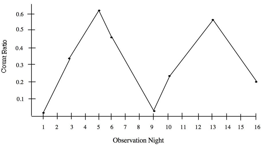
4-29: Period of the Cepheid: 8days.
4-30: Luminosity of Cepheid in solar units: 2000-3000
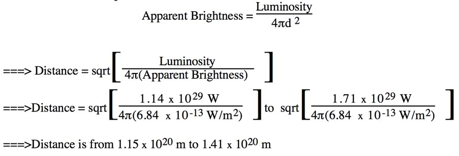
4-31: Luminosity of Cepheid in Watts: 1.14 x 1029 W to 1.71 x 1029 W
4-32: Apparent Brightness of the Cepheid:
Avg. Count ratio of Cepheid to Reference = 0.3
and Apparent Brightness of Reference = 2.28 x 10⁻¹² W/m2 ===>
Apparent brightness of Cepheid = (0.3)(2.28 x 10⁻¹² W/m2) = 6.84 x 10⁻¹³ W/m2
The average Count ratio can be found either by estimating the middle of the cycle and finding the Count ratio there, or by finding the maximum and minimum Count ratio and averaging the two.
One form of the equation to get the apparent brightness of the Cepheid is:
b(v)C = ( CC /Cs ) x b(v)s
where
b(v)C = the apparent brightness of the Cepheid star
b(v)s = the apparent brightness of the standard star
CC/Cs = the average Count ratio of the Cepheid to standard star
There are other equivalent forms and it should be emphasized that any form the student comes up with is fine as long as it gets the job done.
4.33. Distance to the Cepheid in meters:
4.34. Distance to the Cepheid in light years: 12,000-15,000 ly
~{}~
Objectives [] Assessment
Guides for each Chapter: 1 – 2 – 3 – 4 – 5 – 6 – 7 – 8 – 9
Chapter 5. Supernovae
This chapter is designed to teach the techniques used both implicitly in supernova search software and also explicitly by scientists to discover supernovae. The techniques are the same ones used in searching for other variable brightness objects such as Cepheid Variable stars as well as for other objects in the sky such as comets and asteroids.
Investigation 5-1: Finding Supernovae
This investigation starts by breaking down the steps involved so that students work with them one at a time, each time using an image in which only that step is required in finding the supernova. The set of m51fake images, all of which are of galaxy M51, called the Whirlpool Galaxy, have a bright ‘new star’ added, thus their name fake. The m51nor image is a normal image of M51.
The order of steps introduced is as follows:
- Subtracting to reveal a new star that was not seen in the previous, normal image.
- Aligning the two images so they line up before the subtraction is done.
- Adjusting for Brightness Differences due to changing observing conditions before subtracting images, subtracting background sky from both images and multiplying the reference image by the Normalization Factor. In this activity, the images are already aligned.
The four images used in this unit are of supernova SN1990H, the eighth supernova discovered in 1990. In this unit students work with all the steps together that are needed for searching, rather than breaking them down into one step per image as The Techniques Unit does.
Activity I: What Can You Tell By Looking At A Single Image?
One example of settings to enhance the contrast is Min/Max = 895/1650 with no Log scaling. This is an example of settings that work – not the only answer. The point is to bring out the spiral arms but not whiteout the galaxy core.
Activity II: What Can You Tell By Looking At Four Images?
Examples of Min/Max settings to bring out the spiral arms, without Log scaling, are:
snw: 895/1650 snx: 1500/2400 sny: 150/750 snz: 285/985
The supernova is the bright object at (192,256) in snw. It is dimmest in snx, which means this image must be either the first one taken, before the supernova appeared, or the last one, after it had faded away. In fact, it is the latter.
When you use Tile to arrange windows, they are made smaller if necessary to fit all on the screen. To restore, click on the up-arrow or box, called the Maximize button, in the top right corner of the window. In order to have room to expand back to the original window size, the window needs to be away from the bottom and right edges of the screen. For these four image windows, you need to Maximize, or scroll, in order to see the bright star near the bottom right corner of the window.Activity III: Subtracting Images to Find a Supernova
Here are the background sky brightness values using Sky,
and the coordinates of a reference star candidate at about 7 o’clock, using Axes.
This is the information you need for the first two steps, Subtract Sky and Align.
snw: Sky: 943 Center: (118.87, 197.95)
snx: Sky: 1587 Center: (115.29, 114.98)
sny: Sky: 177 Center: (116.18, 111.00)
snz: Sky: 335 Center: (94.95, 90.01)
Here are the Auto Aperture Results for the reference star candidate at about 7 o’clock.
These are the brightness values you need in order to calculate the Normalization factor.
snw: Aperture: (119,107) – Brightness: 23520 – Sky: 943
snx: Aperture: (115,115) – Brightness: 28695 – Sky: 1587
sny; Aperture: (116,110) – Brightness: 19288 – Sky: 176
snz: Aperture: (94,90) – Brightness: 21873 – Sky: 333
Shift
To correct for telescope aim, use the center coordinates from Axes to align each image with the Reference Image. For example, if the star in snw at (118.87, 197.95) is the Reference Star, that same star in snx is at (115.29, 114.98). With snw in the active window, using Shift and entering “-3.58” for the X Offset and “+7.03” for the Y Offset, aligns snw with snx.
After aligning there are two corrections for observing conditions:
Subtract Sky to take out the background sky light.
Normalization
Multiply the image by the Brightness Ratio, called the Normalization Factor,
to correct for haze or high thin clouds.
To calculate the Normalization Factor:
(Reference Star in the Reference Image)/(Reference Star in the New image)
Using the brightness Counts from Auto Aperture and again using the star in snx at (115,115) as the Reference Star, the Normalization Factors are:
Cx/Cx = 28695/28695 = 1
Cx/Cy = 28695/19288 = 1.49
Cx/Cw = 28695/23520 = 1.22
Cx/Cz = 28695/21873 = 1.31
NB: These normalization factors are for revised versions, 9.1/96 and later.
The normalization factors in the earlier versions are the inverses of the ones shown here.
Subtract Images
Here are examples of Min/Max values to adjust the contrast in the subtracted images:
For (snw – snx): -683/242
For (sny – snx): -1000/250
For (snz – snx): -1300/1550.
This adjustment can take a lot of trial and error.
~{}~
Objectives [] Assessment
Guides for each Chapter: 1 – 2 – 3 – 4 – 5 – 6 – 7 – 8 – 9
Chapter 6.
Color, Temperature, and Age of Stars
Investigation 6-1: Observing Color and Temperature
Dimmers and lights available from harware or variety stores. Teachers have suggested that the best equipment for this demo is an aquarium light with a rheostat. You can also use a flame from a Bunsen burner or even a candle, but the burning gases themselves can affect the color of the light as does the temperature of the wick.
Answers:
6.2. What color is the light when the dimmer is on high? blue
6.3. What color is the light at a middle setting? yellow
6.4. What color is the light at the lowest setting? red
6.5. At what setting do you think the light bulb is coolest? low
6.6. At what setting do you think the light bulb is hottest? high
6.7. What color would you expect a very hot star to appear? blue
6.8. Would a very hot star have a high or low B–Vindex? low
6.9. What color would you expect a relatively cool star to appear? red
6.10. Would a cool star have a high or low B-V index? high
6.11. Imagine you could double or even quadruple your distance away from a star.
What would happen to the star’s:
A. Apparent brightness? become less
B Luminosity? unchanged
C. Color? remain unchanged
Investigation 6-2: How Filters Work
If you feel your students need a refresher on the visible spectrum, project a beam of light at an angle through a prism or diffraction grating so that the light emerges in a spectrum. Have students draw the spectrum on a piece of paper, label each color with the first letter in the name of the color, and think of a mnemonic to remember the order of colors. Then have them look at the spectrum through red, blue, and green filters.
Which color looks darkest through the red filter? [blue or green]
Which color looks brightest through the blue filter? [blue]
Describe in words what the filter is doing to light of different colors. [filters let light of only certain colors through]
Optional—look at telescope images:
- Look at the same image using two different lookup tables (in Image menu in SalsaJ).
- Open the image btarg1 and select blue table.
- Then Open the imagebtarg1 again and select red table.
- Move the windows so you have two images side by side, one with a blue star and one with a red star. Please note: you have just instructed the software to color these stars, this is not necessarily related to the true color of the stars.
- Questions:
- For each image, decide which filter makes the star appear brightest, medium, and dimmest.
[Blue lookup table: brightest filter blue; middle filter yellow; dimmest filter red
Red lookup table: brightest filter red; middle filter yellow; dimmest filter blue] - Suppose a red filter is used on the telescope when observing a very blue star. Would the image appear brighter or dimmer or the same as when no filter is used at all? [dimmer]
- Suppose a blue filter is used on the telescope when observing a very blue star. Would the image appear brighter or dimmer or the same as when no filter is used at all? [dimmer; this is tricky. Students may think there will be no change since all of the star’s blue light will still pass through. They need to realize for a blue star that blue is the dominant color emitted, not the only color. This means the blue filter will still block out some of the star’s light, although not as much as the red filter which blocks out virtually all of the dominant color emitted by the star.]
Optional color challenge (students working in groups of four):
One pair in the group will have a colored piece of paper. The other pair, the observers, must estimate the color of the paper by looking at it through various filters. The observers may not see the paper directly until after they have estimated its color. After one pair has a turn at observing, switch roles. For each observing team:
- What was the predicted color of the paper?
- What is the actual color of the paper?
- Describe your technique and logic in predicting the color of the paper.
The point should be emphasized and reemphasized that the filters serve to block out all light except light of the color of the filter. Many students think that a filter changes the color of the light. They also may need to be reminded again and again that the color palette used to display the star has nothing to do with the actual color of the star.
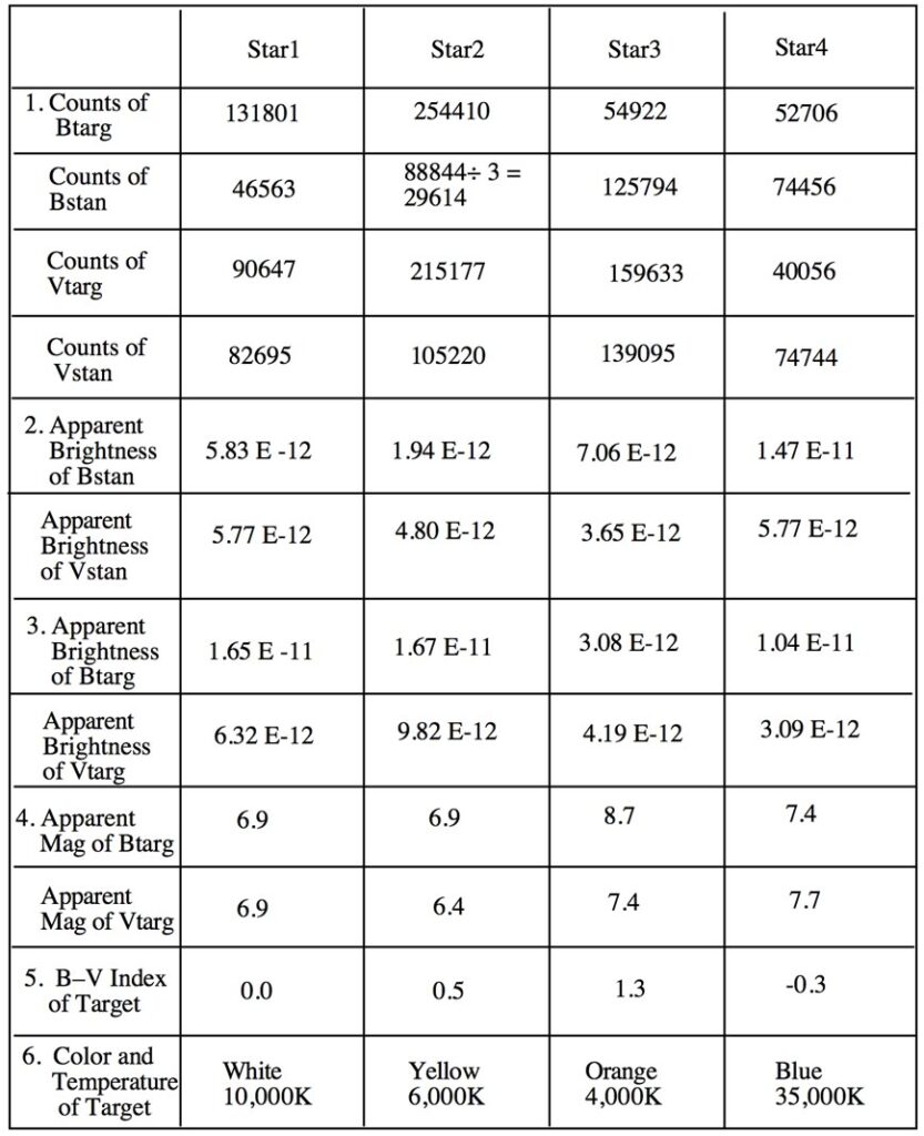
Investigation 6-3: Measuring the Color of Stars
There is a note in the unit about Star B in Blue, but most students will probably miss it the first time. They must divide the Counts for bstan2 by 3 because the exposure time for BStan2 is 3 times that of btarg2, so it gathered 3 times as much light.
Here is an example of the calculations for star1 and the Target Star Brightness table below provides the answers for the rest.
Use Photometry to measure the Counts for the btarg1 and bstan1:
Counts of btarg1 = 131801
Counts of bstan1 = 46563
The apparent magnitude for bstan1 is given as 8.0.
Using the Brightness Conversion Table,
this is equivalent to an apparent brightness of 5.83 x 10⁻¹² Watts/m2.
Use the fact that the Count ratio is equal to the brightness ratio, since the standard star was observed under identical conditions as the target star (with the exception of star 2 as mentioned above) to set up the following equation:
Let
Bt = the apparent brightness of the target star
Bs = the apparent brightness of the standard star
Ct = the Counts of the target star
Cs = the Counts of the standard star
Then Bt /Bs = Ct / Cs
so Bt = (Ct / Cs)Bs
For btarg1, Bt = (131801/46563) 5.83 x 10-12 = 1.65 x 10⁻¹¹
For vtarg1, Bt = (90647/82695) 5.77 x 10-12 = 6.32 x 10⁻¹²
Going back to the Brightness conversion chart, you will find that these values give you the apparent magnitude of btarg1 = 6.9 and the apparent magnitude of vtarg1 = 6.9 as well.
Subtracting the apparent magnitude of vtarg1 from apparent magnitude of btarg1 gives you B-V= 0.0 for star1. Refer to the table provided within the unit to find that this B-V index corresponds to a color of White and surface temperature of 10,000K.
The reason we use magnitudes is because the B-V index is set up on the magnitude scale. All reference material will refer to these values. However, since the magnitude scale is logarithmic and involves calculations that many HOU students are not prepared for, the Brightness Conversion Table allows you to work with the apparent brightness which is a linear scale and allows the use of simple ratios.
Table of Target Star Brightness
Investigation 6-4: HR Diagrams of Star Clusters
The Hertzsprung-Russell (HR) Diagram is a plot that allows determination of stellar type from a star’s color and luminosity. The stellar type yields information about the mass, chemical composition, and age of the star. The surfaces of stars are considered to be blackbody radiators so they follow a Planck spectrum, meaning that their color indicates a unique surface temperature. The process for measuring the color of stars uses images taken through filters. Students will use archived images of known stars to calculate the B–V index, which is obtained from the ratio of brightness through the B and V filters. The relationship between color and temperature is described and students find the temperature of each star.
In order to plot a star on an HR Diagram, its luminosity or absolute magnitude must also be known. The luminosity is proportional to the radius of the star squared and the temperature of the star raised to the fourth power. This means that very large stars can be relatively cool yet have high luminosity (red giants) while very hot stars can be very small and still be reasonably bright (white dwarfs).
HOU DISCUSSION SHEET (from original HOU curriculum)
THE HR DIAGRAM
In the early 1900’s two astronomers were working independently on the classification of stars and came up with very similar results. A Danish astronomer, Ejnar Hertzsprung, plotted stars according to their absolute magnitudes and spectral classes. An American astronomer, Henry Norris Russell, created a plot of luminosity vs. temperature for many stars. Their investigations were seen as roughly equivalent, and the Hertzsprung-Russell (HR) diagram is a result of their findings.
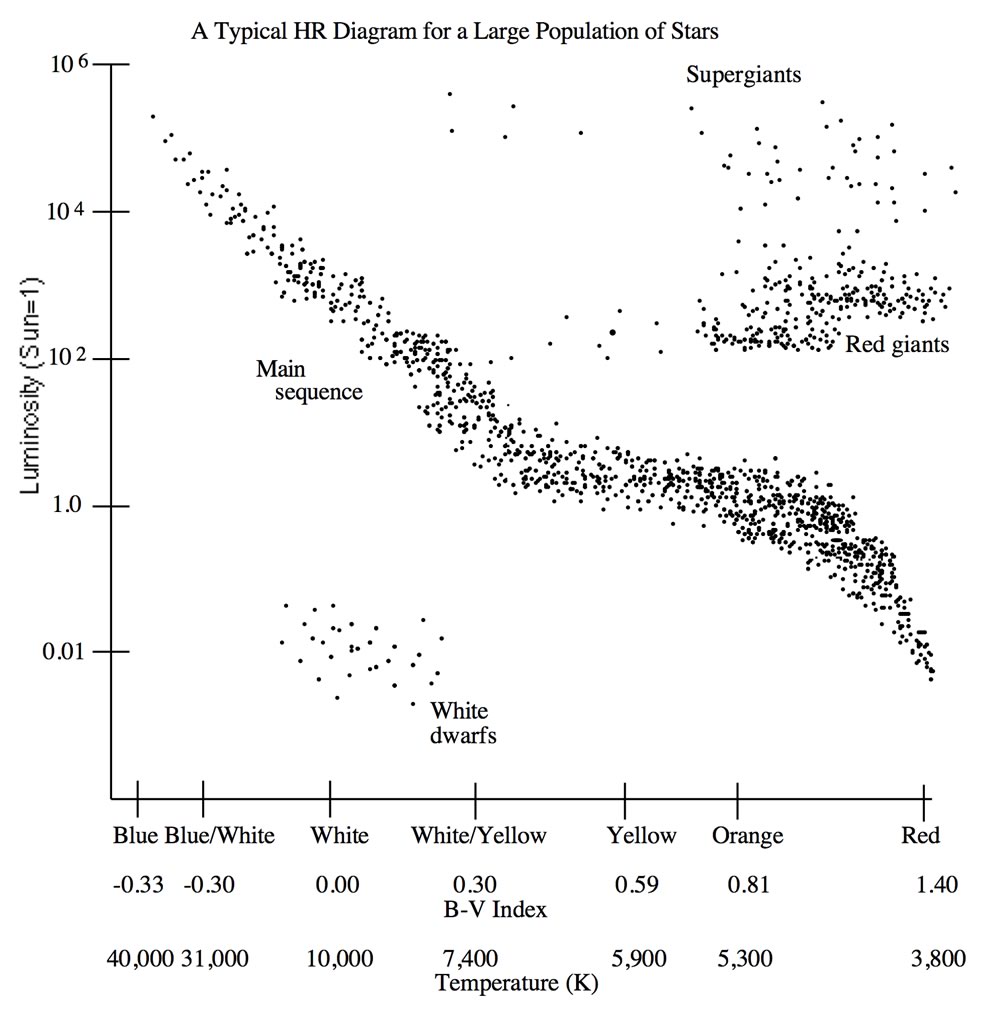
This HR diagram is called a general HR diagram because it is based on stars of all different types from many different regions of the sky. The objective is to show the distribution of various types of stars and their relative quantities. To create a general HR diagram, many stars are observed at a given time, their luminosity and temperature are determined and those values are plotted. The HR diagram can be thought of as a snapshot plot of these stars at one time. A star’s position on the HR diagram is determined by its luminosity and temperature at the time of observation. Since HR diagrams of many different stars, in many different regions, observed at many different times all yield similar distributions, it can be assumed that the general HR diagram describes an average distribution of stars. More specific HR diagrams of a single star cluster are used to determine factors about that cluster such as the type of stars in the cluster and the distance or age of the cluster.
When examining a general HR diagram, notice that the stars are clumped into several groups. The broad line of stars extending from the upper left-hand corner to the lower right is called the main sequence. Most stars on a general HR diagram are on the main sequence because this line represents the luminosity and temperature that exists for most of a star’s life. When a star begins to fuse hydrogen in its core, it assumes its place on the main sequence and stays at that position until its hydrogen fuel runs out and it evolves into a later stage of its life. The main sequence lifetime of a star is generally upwards of 90% of its total lifetime. The temperature, and accordingly the color, of a star during its main sequence period are primarily determined by its mass. High mass stars are very hot so they are blue, while low mass stars are cool and red.
After its hydrogen fuel is depleted, a star contracts and begins to fuse helium in its core. This can occur rapidly or gradually depending on the mass of the star, but in either case it causes the star to expand to a greater radius than that of the main sequence star. During the expansion the star cools considerably. A low mass star that was a yellow or orange main sequence star evolves to a red giant during this expansion period. It is red because it is cool, and it is a giant because it has such a large radius. Similarly, a high mass blue or white main sequence star evolves into a yellow or orange supergiant.
A red giant will undergo yet another phase of evolution where it sheds its outer layers leaving a very dense core of carbon. The outer layers drift off to become what is called a planetary nebula, which is a ring of burning hydrogen that looks like a smoke ring. The dense core is called a white dwarf. It is white because it is very hot, but a dwarf because it has a very small radius. In fact, a white dwarf can have the mass of the sun packed into an object about the size of the Earth. A white dwarf does not have enough mass to initiate carbon burning to produce more energy so it will slowly grow cooler and fade away.
HOU SUPPLEMENTARY ACTIVITY 26 (from original HOU Curriculum)
CLASSIFICATION AND PLOTTING
- Collect data from your classmates, family and neighbors on their age and pulse rate and plot this data on a set of axes. Is there any correspondence between these two characteristics?
- Gather data from your classmates and create a plot of height versus number of siblings.
Is there any correspondence between these two characteristics? - Consider the following pairs of characteristics and predict whether or not there would typically be a correspondence between them:
A. Height and shoe size.
B. Age and eye color.
C. The temperature of a star and its color.
D. The apparent brightness of an object and its distance away.
E. The luminosity of a star and its color. - Collect more data on people’s age and height. Try to get a good distribution of ages. You may want to pool data with others of your classmates. Create a plot with height on the vertical axis and age on the horizontal axis.
- Describe in words the relationship found between people’s age and height.
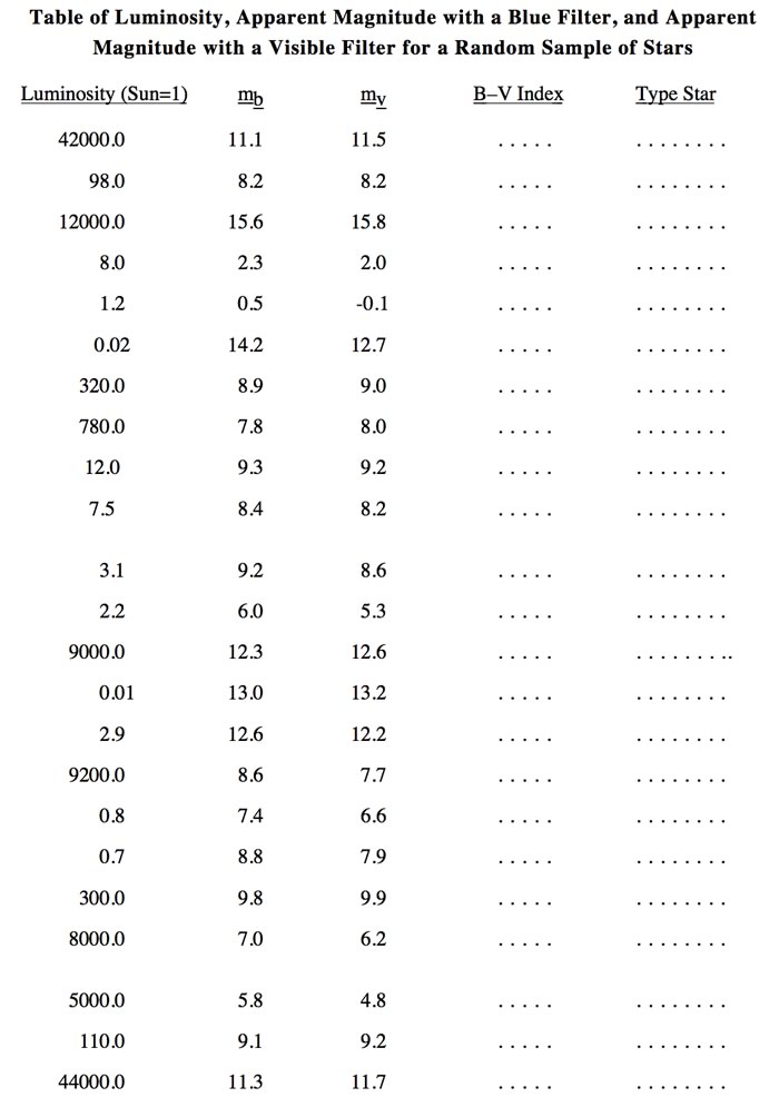
HOU SUPPLEMENTARY ACTIVITY 27
CREATING AN HR DIAGRAM
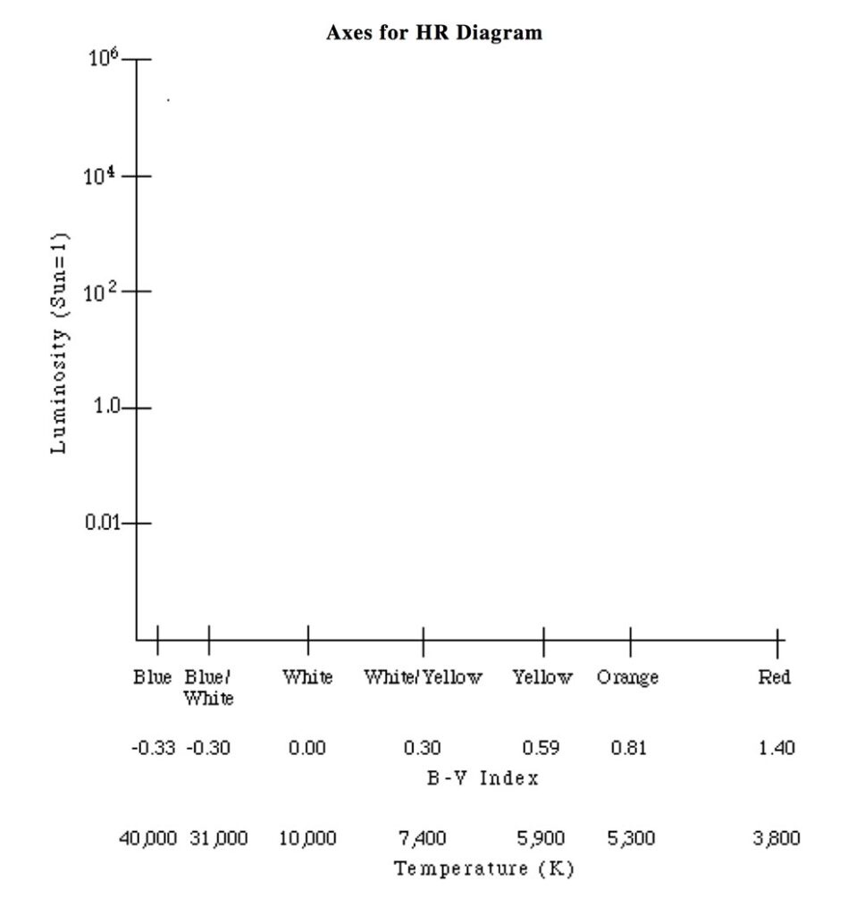
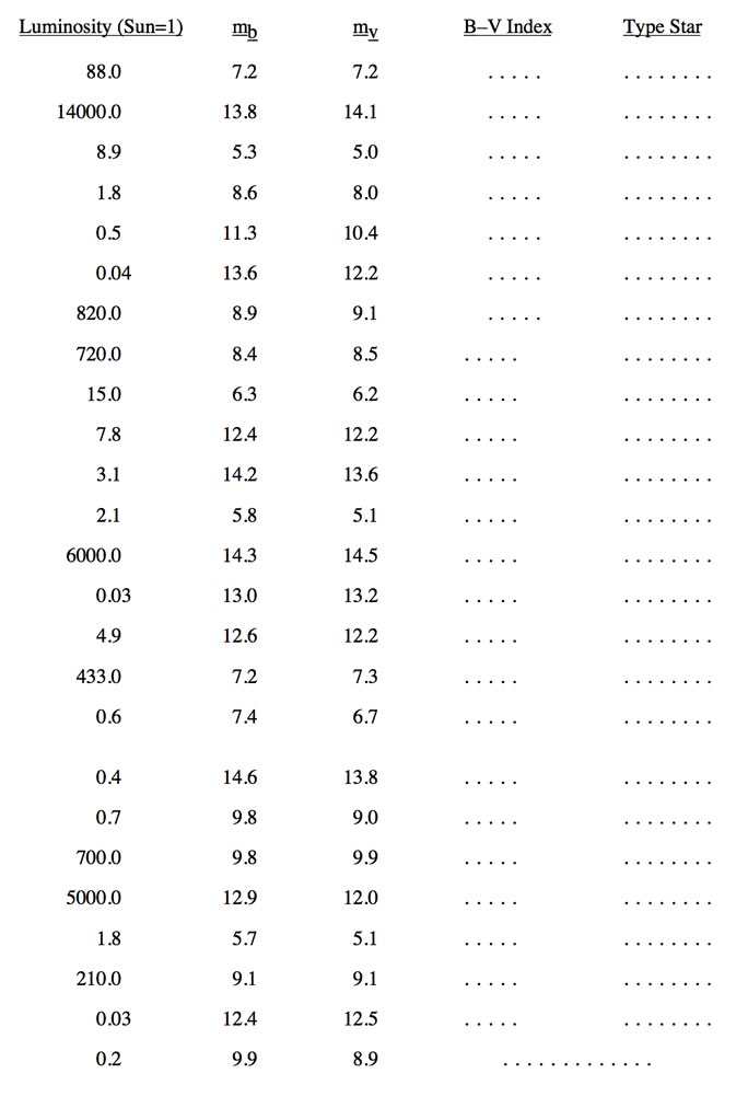
The table below contains the luminosity and color data for 48 stars.
Use the above blank HR Diagram axes to plot the data and create your own HR Diagram.
Be careful to notice that the scale of the plot is not linear.
You will need to calculate the B – V index for each star.
B – V = mb – mv = (magnitude using the B filter) – (magnitude using the V filter)
- Describe any trends or patterns that appear in your plot.
- Lightly circle the regions on the diagram that you would distinguish as isolated groups or clusters. How many different regions do you find?
- Label each region on your diagram indicating its average color and whether it has high or low luminosity.
- Based on your HR Diagram
A. Which stars are hot?
B. Which stars are cool?
C. Which stars are large in radius?
D. Which stars are small in radius? - Use the position of each of your star regions on the HR Diagram to determine the type of star in that region; i.e., main sequence, red giant, supergiant, or white dwarf.
~{}~
Objectives [] Assessment
Guides for each Chapter: 1 – 2 – 3 – 4 – 5 – 6 – 7 – 8 – 9
7. Planet-Star Systems
The first part of this chapter is a series of historical views of the nature of our solar system.
Displacement of the moons of Jupiter on an image can be compared directly by using the ratio of the number of pixels spanned between objects and comparing the velocities of moving objects. In order to translate distance in pixels to a linear dimension across the sky, one needs to know the plate scale of the image and the distance to the object. The plate scale is the angle in the sky subtended by one pixel, and it varies from one CCD to another. Most of the HOU unit images were taken by the CCD camera on the 30″ telescope at Leuschner with a plate scale of 0.67″/pixel, but older Leuschner images (taken with the old CCD) and images from other telescopes will have different plate scales. This information is usually provided in Image Info in a FITS image. Once the angle subtended by the object in the sky is known, the Small Angle Approximation can be used to determine the actual linear dimension of the object in the sky.
HOU Teacher Resource Agents (TRA) Rich Lohman and Jeff Friedman suggested the alternate subtract and add procedure for making a composite image of all six images. As students may discover, only adding the images results in over saturating Jupiter. Adding and subtracting in a more random way solves this problem, but it does make it harder to keep track of which moon is where when two are near each other.
If Jupiter is visible in the night sky for more than six hours, students may want to Request acquire their own images as an alternative to using the set provided. There is an increased sense of ownership when working with your own images. In this case the images need to be aligned to correct for differences in telescope aim before doing any of the adding and subtracting. Find the center coordinates for Jupiter in each of the images and Shift to align each image with the first one in the sequence. The jup5 through 10 images are already aligned.
Activities I and II:
Here is an example of contrast settings for the composite image of the moons after adding #6 to #5, subtracting #7, and continuing to add and subtract:
Min/Max: -300/800 and Log Scaling: No.
Activity III: What Happens to the Moons During Six Hours?
7.7. Image Info (from FITS image header):
| Date | Time (UT) | |
| jup5 | 1992/04/23 | 04:01:02 |
| jup6 | 1992/04/23 | 05:01:20 |
| jup7 | 1992/04/23 | 06:01:10 |
| jup8 | 1992/04/23 | 07:01:12 |
| jup9 | 1992/04/23 | 08:01:17 |
| jup10 | 1992/04/23 | 09:01:24 |
If students are using SalsaJ with JPG images, give them the above times.
[An image Header contains a lot more information than just the date and universal time. The Observatory and observer names are interesting to note; also Right Ascension, RA, and Declination, Dec, and the plate scale.]
One must be careful to keep track of the sequence when making a sextuple image. Starting with jup5, subtract jup6, add jup7, subtract jup8, add jup9, and subtract jup10. The result is a series of alternating white and dark moons corresponding to each moon’s position on its orbit as taken from the six images.
An example of contrast settings that worked well to show the moons is: Min/Max: 304/1286 Log scaling: No.
7.9.
- Moon #1: Moving away from Jupiter, slowing down and stopping; i.e., turning around.
Author’s Note: The distance between images of a moon from hour to hour is a measure of the distance traveled per hour; i.e., the velocity. Using Plot Profile I got changes each hour of 17, 12, 10, 5, and –5 pixels. The average velocity is 49/5 or 10 pixels/hr. The average velocity before turning around is 44/4 or 11 pixels/hr. - Moon #2: Moving away from Jupiter at a steady velocity and in the middle of its orbit, having just emerged from either in front of or behind Jupiter.
Author’s Note: Using Slice I got changes of distance of 18, 18, 18, 18, and 18 pixels. The average velocity is 18 pixels/hr. - Moon #3: Moving away from Jupiter at a fairly steady velocity also.
Author’s Note: Using Slice I got changes of pixel distance of 21, 21, 20, 19, and 18 pixels. The average velocity is 20 pixels/hr. - Moon #4: Moving toward Jupiter at a steady velocity, indicating that its turning point is further out.
Author’s Note: Using Slice I got changes of pixel distance of 13, 13, 13, 14, and 14 pixels. The average velocity is 13 pixels/hr.
10. How I explain the apparent paradox.
In an edge-on view, when a moon is near its turning point most of its motion is away from or toward us. As a moon gets closer to Jupiter more and more of its motion is from left to right or right to left.
Activity IV: Interpreting Your Data.
A potentially frustrating part of this unit is that six hours is not enough information to positively identify each of the four moons. Making an estimate based upon insufficient data, however, is often the best an astronomer can do. In this set of images, Moon #1 turns from moving away to moving toward Jupiter at a place that seems inside positions the other moons are either already beyond or, based on their velocity, will go beyond. Moon #4 comes in from far out, further than it seems any of the other moons can reach. This makes these two moons pretty definitely Io and Callisto, respectively.
Using the data from the table in Activity IV for Europa and Ganymede, it is still unclear which is which. The activity sheet mentions the relationship between orbit radius and velocity. This would seem to be a way to sort them out, but the velocity data is inconclusive on this. Theoretically the moon in the larger orbit moves at a slower velocity. Using data from a reference book:
the ratio of their periods = 2.1 to 1,
and the ratio of their circumferences = 1.6 to 1.
This means the outer moon takes 2.1 times as long to go only 1.6 times the distance covered by the closer moon. To do this the outer moon must move more slowly. With more images in the sequence, the data would be more likely to support this expected relationship.
The following “Notes on the Students” is taken from a paper for a conference in Davis, CA in April, 1995, written by Jeff Friedman, Rick Lohman and Mathew McHugh.
“Students had various problems with shifting the images. Some students had difficulty with the notion of a reference point. That is, students didn’t realize that the center of Jupiter could be used as a reference point for shifting the images so that they would all line up. Students needed to understand that the important thing is the position of the moons with respect to Jupiter. In some cases, students were concerned that they were ‘changing the data’ by shifting, even though they were not changing the critical relationship….
“Secondly, students made arithmetic errors and so when they added all the images up, the moons didn’t appear to be moving in straight lines. When they learned that the moons should line up (either by noticing the results from another group or because a teacher pointed this out), they were faced with the problem of determining which of the images was improperly shifted. This seems to be characteristic of the sort of problem solving required in our image processing based activities. Students learned that they needed to keep careful records of how they manipulated the images and they devised a variety of methods for identifying the misaligned image.
“After successfully superimposing images, students experienced problems in interpretation. Some students assumed that they were viewing the orbital planes from the top, not the side.
“Many students were not interpreting the image as a projection, but were attending to unreliable indicators of distance. For example, some students reasoned that if a moon appeared fuzzier or smaller or if the distance between the moons in successive hours was becoming smaller then that moon was moving further away from the earth.
“From time to time, we would ask students questions to help us understand their thinking and to encourage them to think more meaningfully about the images.”
Determining the Mass of Jupiter
This unit was written by HOU teacher Hughes Pack from Northfield-Mt. Hermon School in Northfield, MA.
Be sure students are clear that the Jupiter images are an edge-on view of circular orbits. It is because the moons are viewed edge-on that the plot of distance versus time is a sine curve. Refer to Sky and Telescope or Astronomy magazines for monthly plots of the moons’ orbits as well as other information pertaining to Jupiter and its moons.
You may want to see the derivation of the equation for determination of the mass of Jupiter.
7.16. Practice Problem: Caution students to be careful about units, such as converting distance to meters and time to seconds. I got 6.02 x 1024 kg, using a hand calculator, which is within 1% of the accepted value, 5.98 x 1024 kg.
7.17. Finding distances from the center of Jupiter (in pixels) will require using the Pythagorean Theorem with the values for the change in x and y. Plot Profile gives a more direct graphic measure of these distances.
7.18. If students do the plot by hand, be sure they plot the moons on the correct side of the line that represents the center of Jupiter. If this graph is done on a graphics calculator or computer, it will be important to use (+) or (-) for distances depending upon whether the moon is to the right or left of Jupiter.
7.19. There is no one way to answer this. The graph shows the change of distance of each of the moons from the center of Jupiter over time.
7.20. The distance is approximately 200 pixels.
7.21. 200 pixels are equivalent to 6.1 x 10⁻⁴ radians.
200 pixels x (0.63″/1 pixel) x ( 1 arcmin/ 60″) x (1 degree/60′) x (1 radian/57.3°)
= 6.1 x 10⁻⁴ radians
7.22. D = (6.63 x 10⁸ km) x (6.1 x 10⁻⁴ radians) = 4.0x 10⁵ km
The actual radius is about 4.22 x 10⁵ km.
7.23. My value from the graph for the time for 1/4 period comes out to be about 9.5 hours. Multiplying this by 4 gives a period of 38 hours.
7.24. An estimate of the error will depend on the values each person gets. The point is to think about each place errors could occur and come up with an estimate. The actual period is 42 hours. I felt that my estimate for 1/4 of the period could have been between 8 and 11 hours depending upon how I drew my curve on the graph and when I estimated the turn-around to occur.
7.25. From the data here, you will get a mass of about 2.0 x 1027 kg.
7.26. Accepted value: 1.9 x 1027 kg. % difference: about 7%.
Investigation 7-2 Asteroid Searches
To become actively involved in asteroid search with your students, see International Astronomical Search Collaboration (https://iasc.cosmosearch.org/)
~{}~
Objectives [] Assessment
Guides for each Chapter: 1 – 2 – 3 – 4 – 5 – 6 – 7 – 8 – 9
Chapter 8. Search for Planets
Here are more exoplanet activities.
NASA Kepler Mission website:
- Transit Tracks
- Animations
- Other Classroom Activities on Planet Finding
- Uncle Al’s Keper Starwheels (a planisphere with locations of naked eye stars with known exoplanets
Laboratory for the Study of Exoplanets (NSF project created by the Harvard-Smithsonian Center for Astrophysics)
Planet Hunters (planethunters.org)
~{}~
Objectives [] Assessment
Guides for each Chapter: 1 – 2 – 3 – 4 – 5 – 6 – 7 – 8 – 9
Chapter 9. Cosmos Ends?
Investigation 9.1 is based on an activity used in conjunction with a planetarium show, How Big Is The Universe. The activity was also made part of the Astronomical Society of the Pacific’s (ASP) Universe At Your Fingertips.